Sequential decision-making

In previous chapter on control certificate functions, we saw how a control input could be synthesized by making minimal adjustments to a desired control in order to satisfy safety (CBF) and performance (CLF) constraints. However, notice that these adjustments are made only for the current time step: how might changing the control input now influence the system’s behavior down the line? Does modifying the desired control in the present have lasting impacts on future performance? Or how does one determine the desired control in the first place?

To address these questions, we need to consider not just individual decisions, but an entire sequence of actions (control inputs), and carefully reason about how each choice can have lasting effects on the future behavior of the system.

Some motivating examples

Going through college: Consider the choices you make as a student: (a) sleeping in and skipping lecture, or (b) waking up early to attend class. In option (a), you experience an immediate reward (or low immediate cost)—extra rest and relaxation. However, this can leave you unprepared for the midterm, requiring much more effort to catch up later, resulting in a lower future reward (or higher future cost). In contrast, option (b) entails a higher immediate cost—waking up early and dedicating energy to attend class—but leaves you better prepared for the midterm, so you need to invest less effort studying later, yielding a higher future reward (or lower future cost).

Which choice is better? That depends on how you weigh immediate rewards or costs against future ones.

We can extend this example: the effort you invest in a prerequisite course (like linear algebra) might influence your performance in advanced engineering courses later on, which in turn could affect your competitiveness when applying for jobs or graduate programs, and so on. Each decision branches into a sequence of future consequences, accumulating over time.

Playing chess: In the game of chess, your moves early in the game affect how your pieces are distributed across the board, and therefore will affect what moves you can make in the future, and ultimately, your ability to win the game. This is a rather challenging sequential decision-making problem because (i) there are many possible moves to make at any turn and many possible board configurations to consider, (ii) there is another player (the opponent) involved and they make moves that we have no control over, (iii) the game is (typically) a long one, involving many moves before a winner is determined, and the payoff of a move right now may not be immediate, but may not come until many moves later.

Healthcare: Suppose you want to treat a patient with a chronic condition. You can offer some treatment options which incur low risk, but which require some amount of effort or time/money cost for the patient, like regular exercise and monthly gym membership, regular therapy sessions that they need to drive to, or eating healthy food which costs more money to buy and time to make. Or, you could offer medium-risk treatment options such as taking a prescription drug that has some potential side effects, or you could offer high-risk surgery which is expensive, time-consuming, and has potential serious side effects. Then the question is: which treatment option should you offer over time as the patient’s condition evolves over time?

These motivating examples involve the need to make a sequence of decisions where each decision will have a consequence—one that will be experienced immediately, and another which will be experienced in the future which will depend on the decision taken right now. Deciding which decision to make ultimately depends on how much you care about the consequences now versus the consequences in the future. This sequential decision making problem is generally a very difficult choice to make for many reasons, but in particular, it is because (i) knowing exactly what the future consequences are is very challenging because there could be so many external influences that could affect it (i.e., stochasticity in the dynamics and disturbances), (ii) there could be many possible situations that arise and it is difficult to consider all the possible cases (i.e., large state space), and (iii) it is difficult to know the true cost/reward of a decision (e.g., how to do you measure the reward of sleeping in versus waking up on time to attend class?).

In the rest of the chapter, we will discuss a principled approach to solving these sequential decision-making problems, and how one may go about solving these problems.

Principle of Optimality

The Principle of Optimality is a cornerstone of sequential decision-making and dynamic programming. It can be expressed in several, but equivalent, ways:

• Any optimal solution to a problem necessarily contains optimal solutions to all of its subproblems.

• If you have an optimal policy, then any “tail segment” of that policy—meaning any actions taken from some intermediate state onward—must itself be optimal for its associated subproblem.

• If you are following an optimal control policy, then no matter where you find yourself along the optimal trajectory, the decisions you make from that point on must continue to be optimal with respect to your current state.

The principle of optimality tells us that, when solving a problem optimally, the sequence of future actions should not depend on the particular sequence of states or actions that led up to the present state—only on the present situation itself. This recursive property makes it possible to break down complex sequential decision-making tasks into simpler, more tractable subproblems. It is exactly this structure that underpins the power of dynamic programming approaches.

By leveraging the principle of optimality, we can systematically compute the best sequence of decisions by solving these subproblems, often using techniques like dynamic programming. By iteratively solving for the tail subproblems, we can then contruct the optimal policy—the optimal control to take from any state.

Pause and Think

Does the Principle of Optimality hold for all types of cost structures? If not, what specific kind of cost structure is required for the principle to apply?

Pause and Think (Answer)

Principle of Optimality is inherently tied to costs with an additive structure. The additivity allows us to break up the problem in a sequence of smaller sub-problems, and ensure that the remaining decisions are not affected by past decisions.

Problem Setup: The Optimal Control Problem

Let’s now precisely formulate the optimal control problem we’re interested in solving. We’ll focus on the classical discrete-time, finite-horizon case for clarity. (In continuous time, the same principles apply, but the main equations become partial differential equations rather than difference equations.)

Let \(x_k\) represent the state and \(u_k\) the control input at time step \(t_k\). Our goal is to determine the optimal sequence of controls that minimizes the overall cost accumulated over a time horizon of length \(N\).

(9)\[\begin{split}\min_{u_{0:T-1}} & \quad \sum_{k=0}^{N-1} J(x_k, u_k, t) + J_N(x_N)\\ \text{subject to} & \quad x_{k+1} = f(x_k, u_k, t_k)\\ & \quad x_0 = x_\mathrm{current}\\ & \quad u_k \in \mathcal{U}(x_k, t_k), x_k \in\mathcal{X}_k\\ & \quad \text{Other constraints...}\end{split}\]

The formulation above defines an optimal control problem. Beyond the basic ingredients—dynamics, initial state, and state and control constraints—there may be additional constraints depending on the specific application. These could include obstacle avoidance, state-triggered constraints, or spatio-temporal requirements, among others.

A key assumption in our setup is that the cost has an additive structure: the total cost is the sum of the stage costs incurred at each time step, \(J(x_k, u_k, t_k)\), plus a terminal cost \(J_N(x_N)\) associated with the final state. This additive structure is crucial, as it enables us to decompose the original problem into a sequence of simpler subproblems, which underpins the dynamic programming approach.

The Value Function (i.e., cost-to-go)

Building on the Principle of Optimality, we can simplify the search for an optimal policy by decomposing it into smaller subproblems that begin at different points along a trajectory. To formalize this recursive approach, we introduce the notion of the value function \(V_\pi: \mathcal{X} \times \mathbb{R} \rightarrow \mathbb{R}\). The value function quantifies the total expected cost (or reward) accumulated from a given state \(x\) at time \(t_k\), when following a given policy \(\pi\) from that point onward. Recall that a policy \(\pi\) is a rule or mapping that gives the control action \(u\) for any state and time, i.e., \(u = \pi(x, t)\).

For the discrete-time, finite-horizon case, the value function is written as:

(10)\[V_\pi(x_k,t_k) = \sum_{k=k}^{N-1} J(x_k, \pi(x_k), t_k) + J_N(x_N)\]

Simply put, we just sum up the total cost from following a policy \(\pi\) from state \(x\), starting at timestep \(t_k\). The value function is interpreted as, and often referred to as, the cost-to-go as it quite literally represents the total future cost from state \(x\).

Naturally, depending on the choice of \(\pi\), your value would be different. So how do we go about picking the optimal policy \(\pi^\star\)?

Optimal value function and policy

To find the optimal policy \(\pi^\star\) (and corresponding optimal value function \(V^\star\)), we simply need to find the policy that minimizes the total cost.

(11)\[\begin{split}V^\star(x_t,t) = \min_{u_{t:T-1}} \sum_{k=t}^{T-1} J(x_k, u_k, k) + J_T(x_T) \quad \text{subject to constraints...}\\ \pi^\star(x_t,t) = \mathrm{arg}\min_{u_{t:T-1}} \sum_{k=t}^{T-1} J(x_k, u_k, k) + J_T(x_T) \quad \text{subject to constraints...}\end{split}\]

To simplify the problem a little bit for ease of notation, let’s remove the constraints for now (except for dynamics constraints).

\[\begin{split} V^\star(x_k,t_k) = \min_{u_{t:N-1}} \sum_{k=k}^{N-1} J(x_k, u_k, t_k) + J_N(x_N)\\ \pi^\star(x_t,t_k) = \mathrm{arg}\min_{u_{t:N-1}} \sum_{k=k}^{N-1} J(x_k, u_k, t_k) + J_N(x_N) \end{split}\]

Even with the constraints removed, while it may become more tractable to solve each individual optimization problem, we would still need to solve this optimization problem for every state in our state space and for all time steps. Hopefully you can see that this will become intractable very quickly, especially for large state spaces and long horizons. Even if it is a relatively small problem and we could enumerate over all possible state, control, and timesteps, it would involve a lot of repeated and wasted computations. This is where the principle of optimality helps!

Bellman equation

Using the principle of optimality, we can break up the defintion of the value function (11) into two parts as follows (again, removing the constraints to make it more notationally simple)

\[ V^\star(x_k,t_k) = \min_{u_{k}} \biggl( J(x_k, u_k, t_k) + \min_{u_{1:N-1}} \sum_{k=k+1}^{N-1} J(x_k, u_k, k) + J_N(x_N) \biggl) \]

We have simply separated out the first term of the summation. But note that the remaining summation term is simply \(V^\star(x_{k+1}, t_{k+1})\), the value function at the next state and next time step! Now, we can rewrite it as,

\[ V^\star(x_k,t_k) = \min_{u_{k}} \biggl( J(x_k, u_k, t_k) + V^\star(x_{k+1}, t_{k+1}) \biggl) = \min_{u_{t}} \biggl( J(x_k, u_k, t_k) + V^\star(f(x_k, u_k, t_k), t_{k+1}) \biggl) \]

So now this optimization problem looks relatively easy to compute! Out of all the possible controls, pick the one that minimizes the sum of the immediate cost \(J(x_k, u_k, t_k)\) and the value at the next state \(V^\star(x_{k+1}, t_{k+1})\). Okay! But first we need to know \(V^\star(x_{k+1}, t_{k+1})\). Well that just looks like the original problem we had, but the time step has progressed by one. So we can repeat what we have above for \(t_{k+1}\). But then we will have the same problem again for \(t_{k+2}\), and so forth.

\[\begin{split} \begin{align*} &V^\star(x_{k+1},t_{k+1}) = \min_{u_{k+1}} \biggl( J(x_{k+1}, u_{k+1}, t_{k+1}) + V^\star(x_{k+2}, t_{k+2}) \biggl)\\ &V^\star(x_{k+2},t_{k+2}) = \min_{u_{k+2}} \biggl( J(x_{k+2}, u_{k+2}, t_{k+2}) + V^\star(x_{k+3}, t_{k+3}) \biggl)\\ &\vdots\\ &V^\star(x_{N-1},t_{N-1}) = \min_{u_{N-1}} \biggl( J(x_{N-1}, u_{N-1}, T_{N-1}) + V^\star(x_{N}, t_N) \biggl) \end{align*} \end{split}\]

Then we notice that at the end of horizon at timestep \(N\), the value at being at state \(x_N\) is given by \(J_N(x_N)\). As such, we have a terminal condition, \(V^\star(x_{N}, t_N)=J_N(x_N)\). Basically, what we have described just now is dynamic programming! and the base case is at timestep \(N\) with \(V^\star(x_{N}, t_N)=J_N(x_N)\). With the base case defined, we can then sweep through the timestep, working backward in time, \(N, N-1,...,2,1,0\).

The Bellman equation essentially describes this recursion,

Bellman Equation (discrete time, finite horizon)

(12)\[\begin{split}&V^\star(x_{k},t_k) = \min_{u_{k}} \biggl( J(x_{k}, u_{k}, t_k) + V^\star(x_{k+1}, t_{k+1}) \biggl), \qquad \text{where} \quad x_{k+1} = f(x_k, u_k, t_k)\\ &\pi^\star(x_{t},t) = \mathrm{arg}\min_{u_{k}} \biggl( J(x_{k}, u_{k}, t_k) + V^\star(x_{k+1}, t_{k+1}) \biggl)\end{split}\]

Pause and think

Although the Bellman equation provides a nice recursive relationship to use, is it straightforward to compute the value function for a general setting, say with nonlinear dynamics, non-trivial constraints, and nonlinear cost terms?

Representing the value function

Depending on the nature of the state and control space, the value function can be represented differently.

• Discrete (finite) state: The value function can be stored in tabular form, with an index for state, and another for time. But if the state space and horizon is very large (e.g., game of chess) then this look-up table would be too large, and in that case, a function approximation (e.g., deep neural network) would be used.

• Continuous state: A tabular form would not make sense since infinitely many rows/cells would be needed. A function approximation (e.g., deep neural network) would typically be used. But for some very simple settings (e.g., Linear Quadratic Regular), the value function is quadratic.

The same can be said for storing the policy.

Another note to mention. We have thus far defined a state-value function where the value is determined purely by the state and timestep. However, another common term is the state-action-value or Q-function which is also used (often in reinforcement learning literature) which considers the action (i.e., control) as an input:

\[ Q_\pi(x_k,u_k,t) = J(x_k,u_k,t_k) + V_\pi(x_{k+1}). \]

Storing the value function in tabular form for discrete state/action/time settings is conceptually straightforward (although the table can quickly become too large to be practical). However, in the case of continuous state and action spaces—even if time remains discrete—the problem becomes much more challenging. Why, in these cases, is the value function so often represented using a deep neural network? Even when dealing with relatively low-dimensional systems and only mildly nonlinear dynamics, why is it so hard to derive a closed-form analytic expression for the value function?

To better understand this challenge, let’s take a closer look at the Bellman equation:

\[ V^\star(x_{k}, t_k) = \min_{u_{k}} \biggl( J(x_{k}, u_{k}, t_k) + V^\star(x_{k+1}, t_{k+1}) \biggr) \]

Suppose that, at timestep \(k+1\), the value function \(V^\star(x_{k+1}, t_{k+1})\) has a “nice” functional form (say, it’s a cubic polynomial). On the right-hand side of the equation, we need to carry out a minimization over \(u_k\). Because the value function and cost are “nice,” perhaps this minimization can also be solved analytically. However, after plugging the minimizing \(u_k\) back in, the resulting function of \(x_k\) may take on a form completely different from that of \(V^\star(x_{k+1}, t_{k+1})\), depending on how the cost \(J\) is structured.

As a consequence, the functional form of \(V^\star(x_{k}, t_{k})\) is generally different from the form we had at the next timestep, \(V^\star(x_{k+1}, t_{k+1})\). Now, when we step back one more timestep to evaluate

\[ V^\star(x_{k-1}, t_{k-1}) = \min_{u_{k-1}} \biggl( J(x_{k-1}, u_{k-1}, t_{k-1}) + V^\star(x_{k}, t_{k}) \biggr), \]

the minimization problem on the right-hand side could require a completely different approach from the previous step. This process repeats itself at each timestep. In other words, the functional form of the value function is generally not preserved as we iterate backward through time using the Bellman equation. This makes it extremely challenging—if not impossible—to obtain a closed-form solution, since the recursive process continuously reshapes the form of the value function.

For this reason, in continuous (or large-scale) problems where analytic solutions are out of reach, we rely on flexible function approximators like deep neural networks to represent value functions across the space of possible states. Of course, this neural network is only an approximation of the true value function.

However, as we will see later, there exists a special class of problems in which the functional form of the value function remains unchanged from one time step to the next. In these cases, it is actually possible to derive a closed-form analytical expression for the value function.

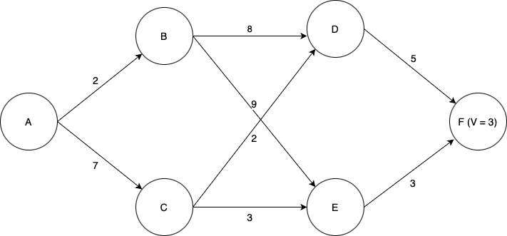
Example: discrete-time, deterministic dynamics, discrete state and control.

Suppose we wish to find the lowest-cost path through the graph shown below. Each node represents a state of some system, and each edge represents an action we can take in a given state to transition to another state. Each edge is labeled with the cost of traversing it (i.e., taking that action), and the final node F is labeled with the known terminal state cost of ending up at that node (in this case, 3). Note then that for this terminal state, the value function \(V\) is equal to three; at first, this is the only state for which we know \(V\).

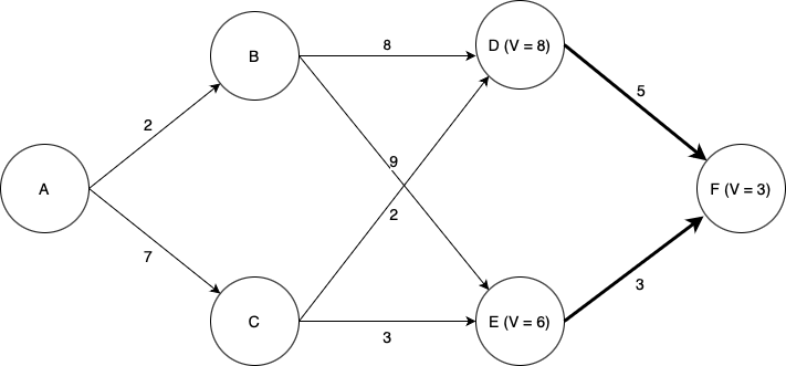
We will use dynamic programming to find the optimal path. First, seeing which states can reach state F, we find that we can now compute \(V\) for each of the states D and E. Since each of these states has only one possible action we can take, this is easy; the value function for each state is equal to the cost of the (one) action we can take in that state, plus the value of the state we end up at (F). Now we can label the graph with the known values of \(V\) at states D and E, as well as highlight the optimal actions to take in states D and E (although there is only one action from each of those states in this case).

Again, we need to determine which states can reach states D and E with a single action. Now things become more interesting. We now need to determine the optimal action and value of \(V\) for each of states B and C. Now we have choices; for example, from state B, we could choose to go to either state D or state E. Which one is best? Again we use the Bellman equation. Let’s look at state B. If we choose to go to state D, we will incur a cost of \(8 + V(D) = 8 + 8 = 16\). If we choose to go to state E we will incur a cost of \(9 + V(E) = 9 + 6 = 15\). Thus we see that the lowest-cost option is to go to state E, and by choosing that action we have \(V = 15\) for state B.

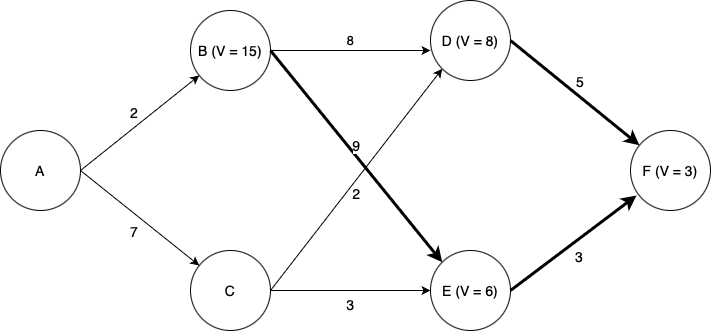
Turning our attention to state C: if we choose to go to state D, we incur a cost of \(2 + V(D) = 2 + 8 = 10\), and if we choose to go to state E we incur a cost of \(3 + V(E) = 3 + 6 = 9\). Thus going to E is the optimal choice, and doing so we have \(V =9\) for state B.

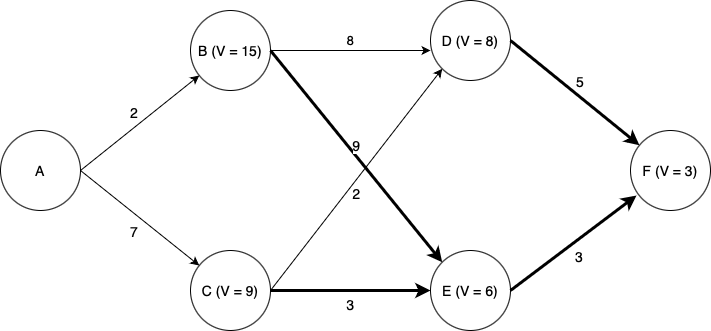
Finally, looking at state A, we see that if we go to state B, we incur a cost of \(2 + V(B) = 2 + 15 = 17\), and if we go to state C we incur a cost of \(7 + V(C) = 7 + 9 = 15\). Thus C is the optimal choice, and \(V = 15\) for state A.

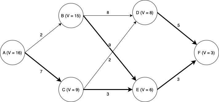
Thus we have computed the optimal path from state A (or from any state onward) to state F.

Note that the computational effort involved scales linearly with the time horizon; considering a time horizon twice as long would only incur twice as much computational effort. A brute-force approach in which we simply enumerate every possible path through the state space and pick the best one would scale exponentially in the time horizon; a time horizon twice as long would square the computation time.

Stochastic dynamic programming

In many real-world scenarios, we cannot predict with certainty which state will result from taking a particular action. That is, given \(x_k\) and \(u_k\), the next state \(x_{k+1}\) is random rather than deterministic.

For example, consider controlling a rocket: the actual thrust generated by the engine for a specific throttle command is subject to variability, so we cannot precisely determine what the rocket’s state will be at a future time. Or imagine playing a game of chess: even with perfect information about the current state (the board configuration), we do not know which move our opponent will make in response to ours. We might have some idea about the likelihood of certain moves based on experience or an understanding of our opponent, and indeed, part of advanced chess strategy is to guide opponents toward desirable actions—but ultimately, the future is uncertain.

To address this inherent stochasticity, we turn to methods that can properly account for uncertainty. A widely used approach is dynamic programming, where instead of optimizing the value function \(V(x, t)\) directly, we work with the expected value of the value function, denoted \(\mathbb{E}[V(x, t)]\).

Moreover, in such settings the cost function itself may depend not only on the current state and control, but also on the resulting next state. Because the next state is uncertain, the incurred cost is likewise a random variable.

Adapting the previous notation slightly to account for stochasticity in the problem:

• Instead of dynamics \(x_{k+1} = f(x_k, u_k, t_k)\), we consider state transition probabilities where \(x_{k+1} \sim p(x_{k+1} \mid x_k, u_k)\).

• Instead of a cost \(J(x_k, u_k, k)\), we consider \(J(x_k, u_k, x_{k+1}, t_k)\).

Stochastic Bellman Equation (discrete time, finite horizon)

(13)\[\begin{split}&V^\star(x_{k},t_k) = \min_{u_{k}} \biggl( \mathbb{E}_{x_{k+1}\sim p(x_{k+1} \mid x_k, u_k)}[ J(x_{k}, u_{k}, x_{k+1}, t_k) + V^\star(x_{k+1}, t_{k+1})] \biggl), \\ &\pi^\star(x_{k},t_k) = \mathrm{arg}\min_{u_{k}} \biggl( \mathbb{E}_{x_{k+1}\sim p(x_{k+1} \mid x_t, u_k)}[ J(x_{k}, u_{k}, x_{k+1}, t_k) + V^\star(x_{k+1}, t_{k+1})] \biggl)\end{split}\]

Example: discrete-time, stochastic dynamics, discrete state and control.

Suppose we wish to find the lowest-cost path through the graph shown below. Each node represents a state of some system, and each edge represents a possible transition between states. Note that in the stocastic case, state transitions do not correspond directly to actions. In this example, we assume that in each state, there are two actions we can take: “Action 1” and “Action 2”. Each transition edge is labeled with two numbers; the first is the probability of that state transition occuring if we take Action 1, and the second is the probability of that state transition occuring if we take Action 2. The value of ending up in either of the two final states is marked in the graph. Taking Action 1 costs 1 unit of value, and taking Action 2 costs 2 units of value. We seek to find a sequence of actions that maximizes the expected total value of the path.

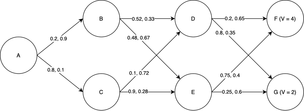
We will use dynamic programming to find the optimal path. First, we must find \(V\) for each of the states D and E. Starting with state D: the expected total value if we take Action 1 is \(0.2\times V(F) + 0.8\times V(G) - 1 = 0.2\times4 + 0.8\times 2 - 1 = 1.4\). The expected total value if we take Action 2 is \(0.65\times V(F) + 0.35\times V(G) - 2 = 0.65\times 4 + 0.35\times 2 - 2 = 1.3\). Of these, 1.4 is greater, and so the optimal action to take in state D is Action 1, and \(V(D) = 1.4\). Performing the same process for state E, we find that the optimal action is again Action 1, and \(V(E) = 2.5\).

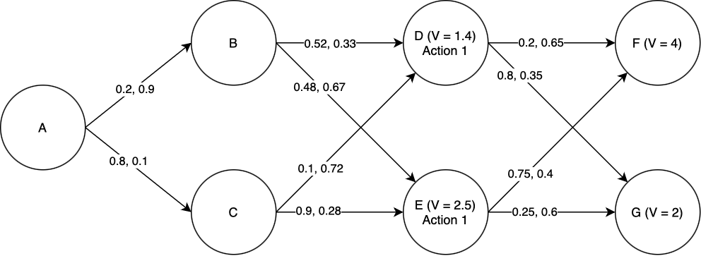
Now we proceed to states B and C. For state B: if we take Action 1, the expected total value is \(0.52\times V(D) + 0.48\times V(E) - 1 = 0.52\times 1.4 + 0.48\times 2.5 - 1 = 0.928\). If we take Action 2, the expected total value is \(0.33\times V(D) + 0.67\times V(E) - 2 = 0.33\times 1.4 + 0.67\times 2.5 - 2 = 0.137\). Of these, 0.928 is greater, and so Action 1 is the optimal action and \(V(B) = 0.928\). By a similar process we find the optimal action for state C, and also \(V(C)\).

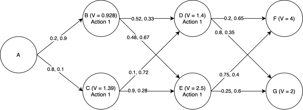
Finally, the same procedure lets us compute the optimal action at state a, and also \(V(A)\).

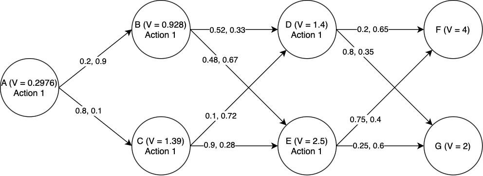
Thus we have computed the optimal actions to take from state A (or from any state onward) to the end.

Note that for this particular case, Action 1 was always the best action to take (turns out it’s hard to make up an example that you know in advance will give “interesting” results). But this highlights the power of dynamic programming: imagine how hard it would be to tell what the right action is in each state just by looking at the graph, and not going throught the stochastic dynamic programming process.

Infinite time horizon dynamic programming

Often we are interested in problems with an infinite time horizon. For example, suppose we are designing a stabilization system for a cruise ship, to reduce rolling due to waves. The cruise ship will put out to sea, activate the stabilization system, and leave it running “indefinitely”, or at least until it gets back to port. Since we don’t know how long the stabilizer will have to run (and in any case it will run for a very long time on each journey), we can just assume it will run “forever”. In cases like these, infinite-horizon dynamic programming is useful.

In infinite-horizon dynamic programming, it no longer makes sense to consider a terminal state cost, since there is no terminal state. Instead, we use the infinite-horizon Bellman equation, which includes a “discount factor” \(\gamma\) multiplying \(V(x_{t+1}, t+1)\), where \(0 < \gamma < 1\):

It also does not make sense to keep track of timestep in the infinite horizon case since the horizon is, well, infinite. Keeping track of what the value is at timestep, say, 1000000 versus time step 100 is not particularly useful since the horizon is infinite. As such, we drop the time argument in our value function definition.

Infinite-Horizon Bellman Equation (discrete time)

(14)\[\begin{split}&V^\star(x) = \min_{u} \biggl( J(x, u) + \gamma V^\star(f(x,u)) \biggl), \qquad \text{where} \quad x_{t+1} = f(x_t, u_t)\\ &\pi^\star(x_{t}) = \mathrm{arg}\min_{u} \biggl( J(x, u) + \gamma V^\star(f(x,u)) \biggl), \qquad \text{where} \quad x_{t+1} = f(x_t, u_t)\\\end{split}\]

\[\begin{split} \begin{align*} &V^\star(x) = \min_{u} \biggl( J(x, u) + \gamma V^\star(f(x,u)) \biggl), \qquad \text{where} \quad x_{k+1} = f(x_k, u_k)\\ &\pi^\star(x) = \mathrm{arg}\min_{u} \biggl( J(x, u) + \gamma V^\star(f(x,u)) \biggl), \qquad \text{where} \quad x_{k+1} = f(x_k, u_k)\\ \end{align*} \end{split}\]

The discount factor plays a crucial role in infinite-horizon dynamic programming. Most importantly, it guarantees that the value function remains finite: without discounting, the total cost could diverge if future cost terms do not decrease rapidly enough. The discount factor ensures that future costs contribute less and less to the total value as time progresses.

Practically, the discount factor also affects how the optimal policy balances immediate and future outcomes. A lower discount factor \(\gamma\) (closer to 0) makes the policy focus more on immediate rewards or costs, while a higher \(\gamma\) (closer to 1) places greater emphasis on long-term consequences. The choice of discount factor thus reflects how much we care about near-term versus far-term outcomes.

It is also possible to include a discount factor in the finite horizon case. It has the same interpretation, but there isn’t a risk of the value being infinite since the time horizon is finite.

But how do we actually compute the value function for an infinite-horizon problem? At first glance, this seems challenging: dynamic programming typically works by moving backwards through time, but with an infinite horizon, there is no terminal time to start from, nor can we perform infinitely many iterations!

This is precisely where the discount factor \(\gamma\) (with \(0 < \gamma < 1\)) becomes essential. The presence of this discount factor ensures that the value function \(V(x)\) converges as we iterate the dynamic programming updates: with each iteration, the values approach a limiting solution. Crucially, we do not need to specify a terminal value—no matter how we initialize \(V(x)\), the effect of that initial guess vanishes over time due to the discounting, and the value function converges to the same result. In practice, we simply pick an arbitrary starting point for \(V(x)\) and iteratively apply the Bellman update until the changes become sufficiently small (as measured by a convergence tolerance \(\epsilon\)).

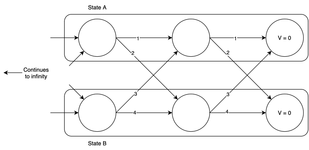
Example: discrete-time, deterministic dynamics, discrete state and control, infinite-horizon.

Suppose we have a discrete-time system with two states, A and B. At each time step we can remain in the state we’re in, or transition to the other; each action has a certain cost. A graph representation of this system is shown below, at some imaginary “end of time” from which we initialize the DP process; you can imagine that the graph extends infinitely to the left. The graph edges represent the possible state transitions from one time step to the next, and are labeled with their costs. We seek to find the optimal action in each state to minimize the total cost until the end of time, using the infinite-horizon Bellman equation. We arbitrarily assign \(V(A) = V(B) = 0\) at the “end of time”, and in this case we will consider a discount factor of \(\gamma = 0.9\).

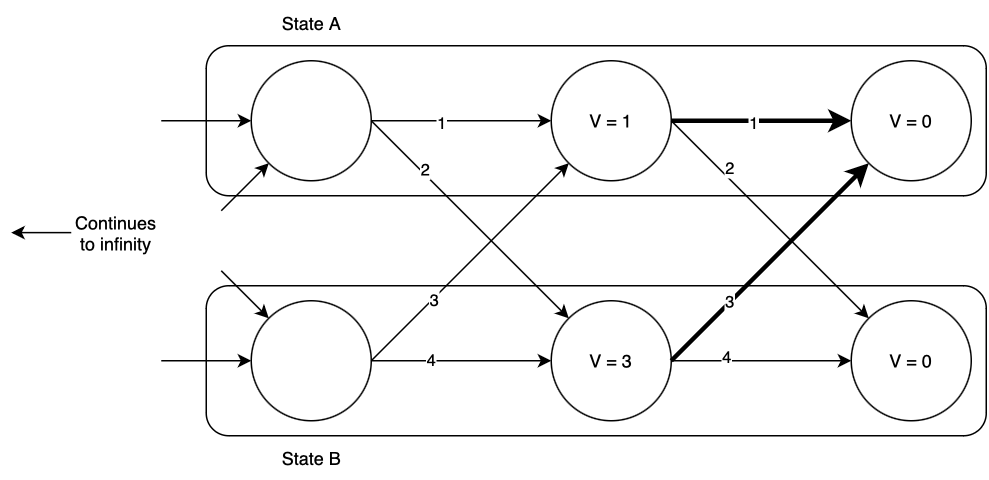
Now we begin the dynamic programming process. Consider state A, one time step back from the “end of time”. What is the optimal action, and value of \(V(A)\)? If we remain in state A, we will incur a total cost of \(1 + 0.9\times 0 = 1\), and if we transition to state B, we will incur a total cost of \(2 + 0.9\times 0 = 2\). Of the two, remaining in state A has the lower cost, so that is the optimal action, and at this time step \(V(A) = 1)\). Now consider state B: if we remain in state B, we will incur a total cost of \(4 + 0.9\times 0 = 4\), and if we transition to state A we will incur a total cost of \(3+0.9\times 0 = 3\). Thus we should transition to state A, and at this time step \(V(B) = 3\). The optimal transitions are highlighted below.

Now we move one time step back and repeat the process, finding again that the optimal action is to remain in state A if you’re already there, or to transition to state A if you’re in state B. The optimal values of \(V(x, t)\) and optimal actions are shown below.

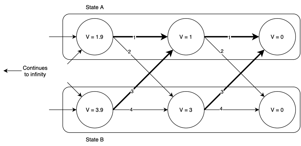
Notice that as we go backward in time, \(V(x)\) increases; however, it appears to be slowing down. Going one time step back from the end of time, \(V(x)\) increased by more than it did when we went one step further. This pattern will continue until eventually \(V(x)\) converges. In this case, the values that \(V(x)\) converges to are \(V(A) = 10, V(B) = 12\). (Try this yourself! Write some code to iteratively compute these values. Also try different initializations of \(V(x)\) other than zero; does it make a difference?)

Hamilton-Jacobi-Bellman equation

So far, we have considered a discrete-time setting. What about the continuous-time setting? We can derive the continuous-time case by casting the continuous time problem into a discrete-time problem with timestep \(\Delta t\) and let \(\Delta t\rightarrow 0\) and see what we get as a result of taking that limit. With the continuous-time setting, our dynamics are \(\dot{x} = f(x,u,t)\) and the cost is \(\int_0^T J(x,u,t) dt + J_T(x(T))\). Note that the cost is an integral, but to “convert to discrete-time”, the cost over a \(\Delta t\) time step is approximated to be \(J(x,u,t) \Delta t\).

Considering we are at timestep \(t\) and we consider a timestep size of \(\Delta t\), the Bellman equation can be written as,

\[ V^\star(x(t),t) = \min_{u(t)} \biggl( J(x(t), u(t), t)\Delta t + V^\star(x(t+\Delta t), t+\Delta t) \biggl) \]

Now we rearrange the terms and take the limit \(\Delta t\rightarrow 0\).

\[\begin{split} \begin{align*} 0 &= \min_{u(t)} \biggl( J(x(t), u(t), t)\Delta t + V^\star(x(t+\Delta t), t+\Delta t) - V^\star(x(t),t) \biggl)\\ 0 &= \min_{u(t)} \biggl( J(x(t), u(t), t) + \frac{V^\star(x(t+\Delta t), t+\Delta t) - V^\star(x(t),t)}{\Delta t} \biggl), \qquad (\div \Delta t)\\ \lim_{\Delta t \rightarrow 0} 0 &= \lim_{\Delta t \rightarrow 0} \min_{u(t)} \biggl( J(x(t), u(t), t) + \underbrace{\frac{V^\star(x(t+\Delta t), t+\Delta t) - V^\star(x(t),t)}{\Delta t}}_{\text{Total derivative}} \biggl)\\ &= \min_{u(t)} \biggl( J(x(t), u(t), t) + \frac{\partial V^\star}{\partial t}(x,t) + \nabla V^\star(x,t)^Tf(x,u,t) \biggl)\\ 0 &= \frac{\partial V^\star}{\partial t}(x,t) + \min_{u(t)} \biggl( J(x(t), u(t), t) + \nabla V^\star(x,t)^Tf(x,u,t) \biggl) \end{align*} \end{split}\]

The resulting expression is a partial differential equation where the solution is the value function. We have \(V(x,T) = J_T(x)\) as a boundary condition, and we must solve the PDE backward in time to get the value function over all entire time horizon.

Hamilton-Jacobi-Bellman Equation (continuous-time, finite horizon)

(15)\[\begin{split}0 &= \frac{\partial V^\star}{\partial t}(x,t) + \min_{u(t)} \biggl( J(x(t), u(t), t) + \nabla V^\star(x,t)^Tf(x,u,t) \biggl)\\ V^\star(x,T) &= J_T(x)\end{split}\]

Solving the HJB is Hard!

While the Hamilton-Jacobi-Bellman (HJB) equation gives a powerful and general framework for finding optimal policies, actually solving the HJB equation is, in most cases, extremely challenging or even intractable. The main reasons are:

• The HJB is a nonlinear partial differential equation (PDE); such PDEs can be very difficult to solve analytically except for the simplest systems (like linear-quadratic problems).

• For most practical systems, the dimension of the state space is high; since the value function depends on the entire state, solving the PDE numerically suffers from the curse of dimensionality—computational costs grow exponentially with state dimension.

• Boundary conditions, nonlinearity, and constraints make analytical solutions impossible in almost all but toy problems.

For these reasons, most practical optimal control algorithms use either approximate methods (such as value/policy iteration, model predictive control, or approximations from learning-based methods) or try to restrict the class of problems so that the HJB admits a tractable solution (e.g., LQR, specific classes of stochastic control, etc.). Still, the HJB provides critical insight into the structure of optimal control solutions, even if it is rarely solved exactly!

Next, we will learn about the Linear Quadratic Regulator (LQR). While you may have learned about it previously, and possibly introduced in a different way, we will consider the LQR problem as a special case of the Bellman and HJB equation for which solve them in closed form is possible!!

Additional reading

• Chapter 4: Reinforcement Learning: An Introduction (2nd Ed) by Richard S. Sutton and Andrew Barto

• Chapter 7: Underactuated Robotics Course Notes by Russ Tedrake

• Dynamic Programming and Optimal Control by Dimitri P. Bertsekas (No free online version, but there are some online videos available.)